The beginning of 2025 marked the 350th anniversary of the hairspring, the invention that made portable precision timekeeping possible. To commemorate the occasion, we published a series of deep dives covering the disputes around its invention, the evolution of spring materials over the years and the finer rules of forming Breguet overcoils. This final instalment examines isochronism.

Some initial definitions and considerations

A proper and universal definition of isochronism is: the property of an oscillatory system to maintain the same period of vibration despite variation in environmental factors. This implies that a vibrational system’s behaviour is inherent and external factors should not influence its frequency. 

A few basic terms help frame the discussion. The period, measured in seconds, is the time taken for the oscillator to travel from one extreme position, through equilibrium, and back again. Frequency, measured in Hertz, is the inverse of the period; a system with a constant period can serve as a stable timebase.

The amplitude is the distance swept by the oscillator from the equilibrium point to its extreme position. In practical terms, when saying that a sprung balance has an amplitude of 330°, it means the balance wheel rotates a full 330° in one direction from its equilibrium point before swinging back. 

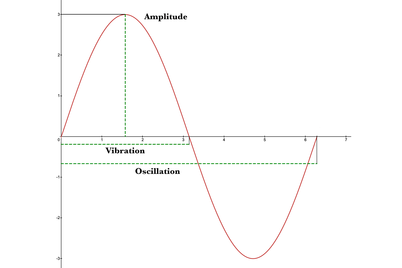
Figure I. Anatomy of a sinusoidal wave.

In watchmaking parlance, isochronism means that an oscillator keeps the same period, regardless of its amplitude. This simplified definition foregoes the broader set of “external factors” and instead focuses just on the amplitude characteristic of the oscillator. Physically it is quasi-impossible for a real system to always retain the same vibration period, since there are always resisting forces and imperfections that work against the ideal conservation of energy and dampen the oscillator.

This is why any mechanical oscillator needs to be cyclically recharged by an escapement mechanism, which restores the lost energy to the system. While the oscillator loses energy at a constant pace, the escapement (its power dependent on the mainspring) restores energy in a non-constant manner. It means that sometimes the escapement provides higher or lower energy to the oscillator, depending on the state of mainspring charge. 

An inconsistent recharge coming from the escapement influences the oscillation amplitude. When the mainspring barrel is fully wound up, it exerts a strong torque onto the going train and consequently onto the oscillator. As the mainspring unwinds, its torque decreases in a quasi-linear fashion, thus supplying less and less energy to the oscillator. 

As the mainspring weakens, the amplitude tends to decrease. This makes it essential for the oscillating system to be as isochronous as possible so that reduced amplitude does not degrade timekeeping.

This article considers why the sprung balance has the potential to be inherently isochronous, whereas other systems, like the pendulum, do not.

A bit about the physics of oscillators

Before going into the real-world details of oscillating organs, let’s look at the simplest oscillator model: the conservative harmonic oscillator. A purely theoretical model, the harmonic oscillator doesn’t encounter resisting forces — so there is no need for an escapement. Simple harmonic oscillators are usually modelled as mass-spring systems. 

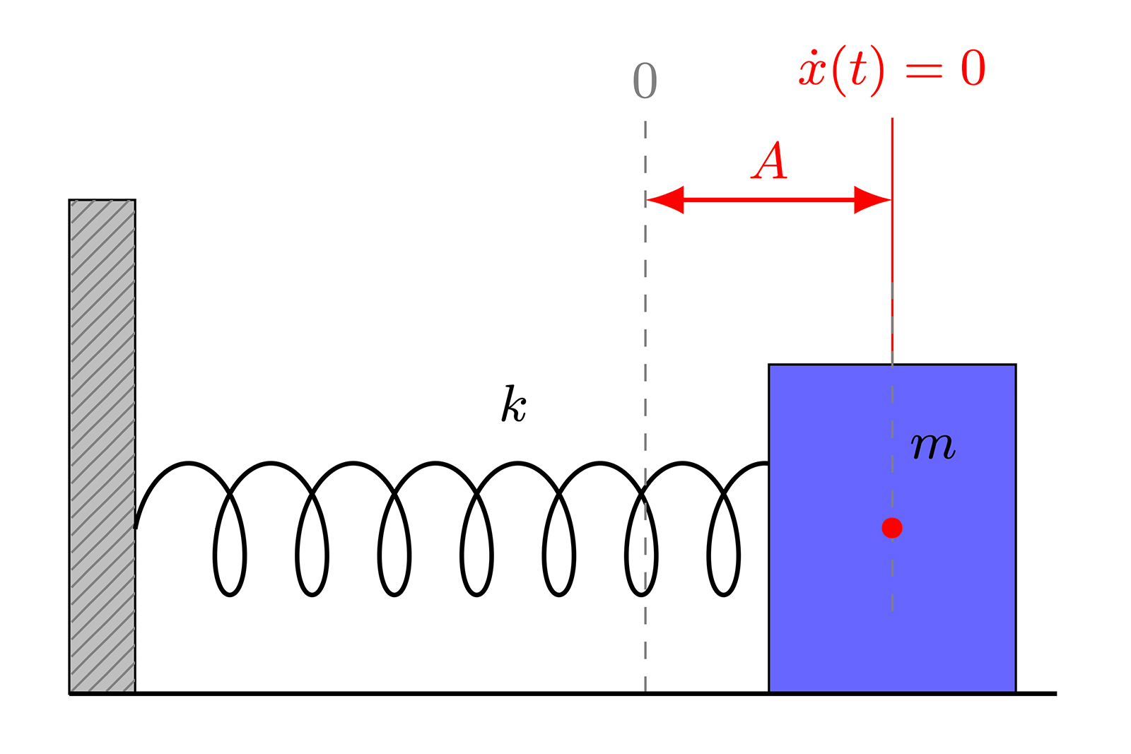
Figure II a. The mass is kept still at a positive distance A from the equilibrium point.

The theoretical model is released from rest from a chosen maximal position A at time t=0 (Figure II a). As the the spring is tensioned, it pulls back at the mass from rest and makes it overshoot the equilibrium position (the particular position where the spring is neither in extension nor in compression). At one point the compressed spring stops the mass and pushes it back towards equilibrium. Since there are no resisting forces in this model (i.e. no friction or air drag), the oscillation goes on infinitely around the equilibrium position, from -A to +A (Figures II b & c). 

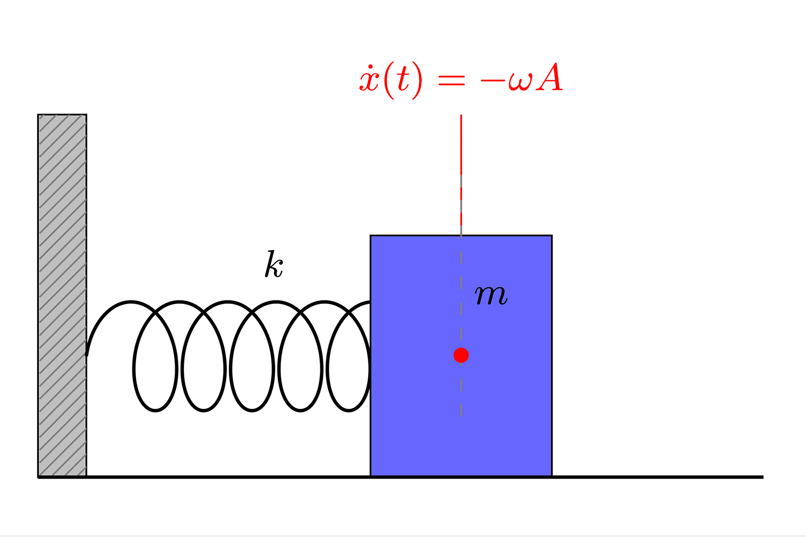
Figure II b. The mass reaches its maximum velocity at the equilibrium point.

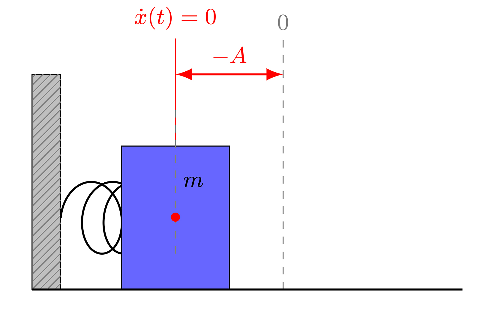
Figure II c. The other maximum displacement position at -A; the block has a null velocity and the spring is compressed to the max.

The known equation of motion of the harmonic oscillator is in the first row of Figure III. There are only three terms involved: displacement r, its second derivative acceleration and a squared constant called pulsation. 

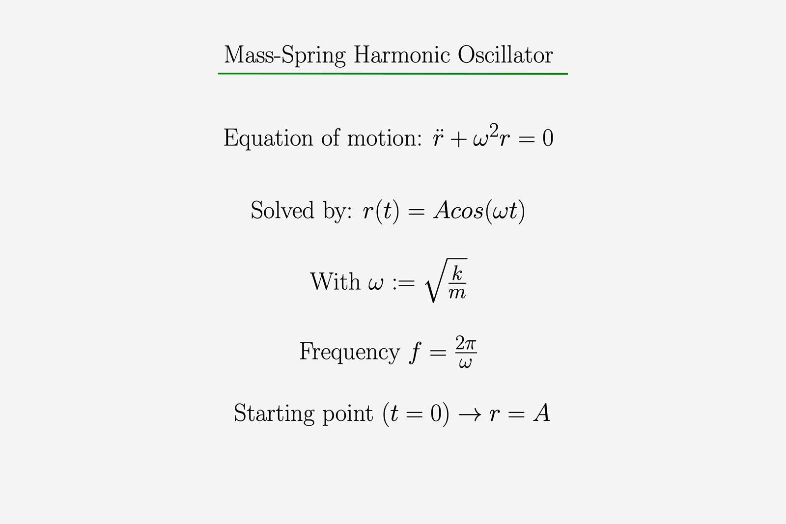
Figure III. Equations governing the harmonic oscillator.

The differential equation is satisfied by the particular solution in the second row. It gives us the system’s position with regards to time. At time t=0 we get that the position is the amplitude A, which satisfies our model.

The important takeaway here is that the harmonic oscillator and every other system which is governed by this equation of motion is isochronal. Pulsation ω in this case is the square root of the spring stiffness k over the mass m. This tells us that the oscillator is fully independent of the amplitude. Regardless of the choice of A, the system will have the same eigenfrequency (its own natural frequency), so even if the amplitude varies over time, the timing won’t be affected. In other words the system will go from -A to zero and over to +A in the same time period, regardless if we double or triple the amplitude.  

With that foundation, we can now turn to the pendulum and the sprung balance and examine how both compare to the ideal model.

The flawed pendulum

Most stationary precision clocks traditionally relied on large, heavy pendulums, which can achieve remarkable accuracy under controlled conditions. Yet pendulums are not inherently isochronous.

Pendulums were considered isochronous for a very long time. Galileo Galilei (1564-1642) famously used his own heartbeat to time the swings of a cathedral’s chandelier, noticing how the vibrations took the same time regardless of the swept distance. His observation was only partly true. 

Much later, the Dutch scientist and father of the hairspring Christiaan Huygens (1629-1695) developed the cycloid pendulum theory, claiming that rigid pendulums were not isochronous. Huygens’ published work on the subject Horologium Oscillatorium is an elegant exhibit of mathematics and geometric reasoning. His hypothesis can be validated today by way of differential calculus. At that point however this method was yet to be invented and was thus unavailable to him, making his geometric reasonings all the more fascinating. 

So if pendulums are not inherently isochronous, how come they are found in so many precision clocks? After all, Rifler regulator clocks and Shortt-Synchronome pendulums remain among the most accurate non-quartz, non-atomic timekeepers ever made.

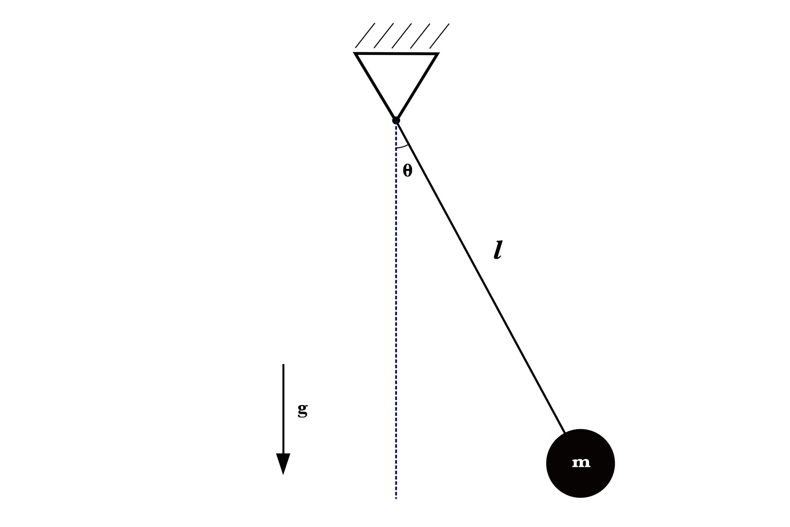
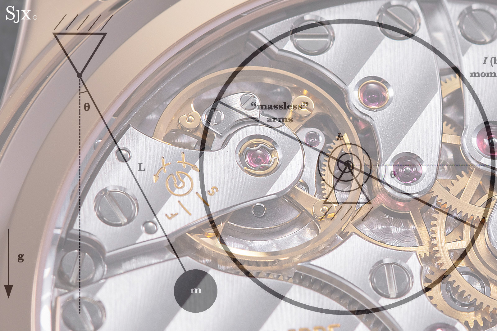
Figure IV. Simple free-body model of a swinging pendulum.

To answer this question, let’s take a look at the free swinging pendulum. Every real pendulum can be modelled mathematically in a simple way: the real weighted rod and mass can be replaced by a massless rigid rod and point mass. This setup is familiar to physics students who get to study harmonic oscillators. We will treat the pendulum in the same manner as the spring-mass model from the previous section: no resistive forces acting on the system. 

Commonly the period of a swinging pendulum is taught to be only dependent on the gravitational acceleration constant g and the pivoting length l of the pendulum, from fulcrum to the center of mass. This is inaccurate and we can easily spot why. 

Using Lagrangian (or Newtonian) mechanics we can quickly retrieve the equation of motion for a free, non-dampened pendulum. As shown in the first row in Figure V, the equation of motion involves the pendulum’s polar inertia moment around the pivot point I, its mass, length and the gravity acceleration constant g. The second row shows the same equation in its final form. 

The equation looks almost identical to the harmonic oscillator equation in Figure III, save for the sine function replacing the simple angular displacement. Even if we set the pulsation ω to be the square root of g over l, we still can’t easily solve the differential equation in a clean manner.

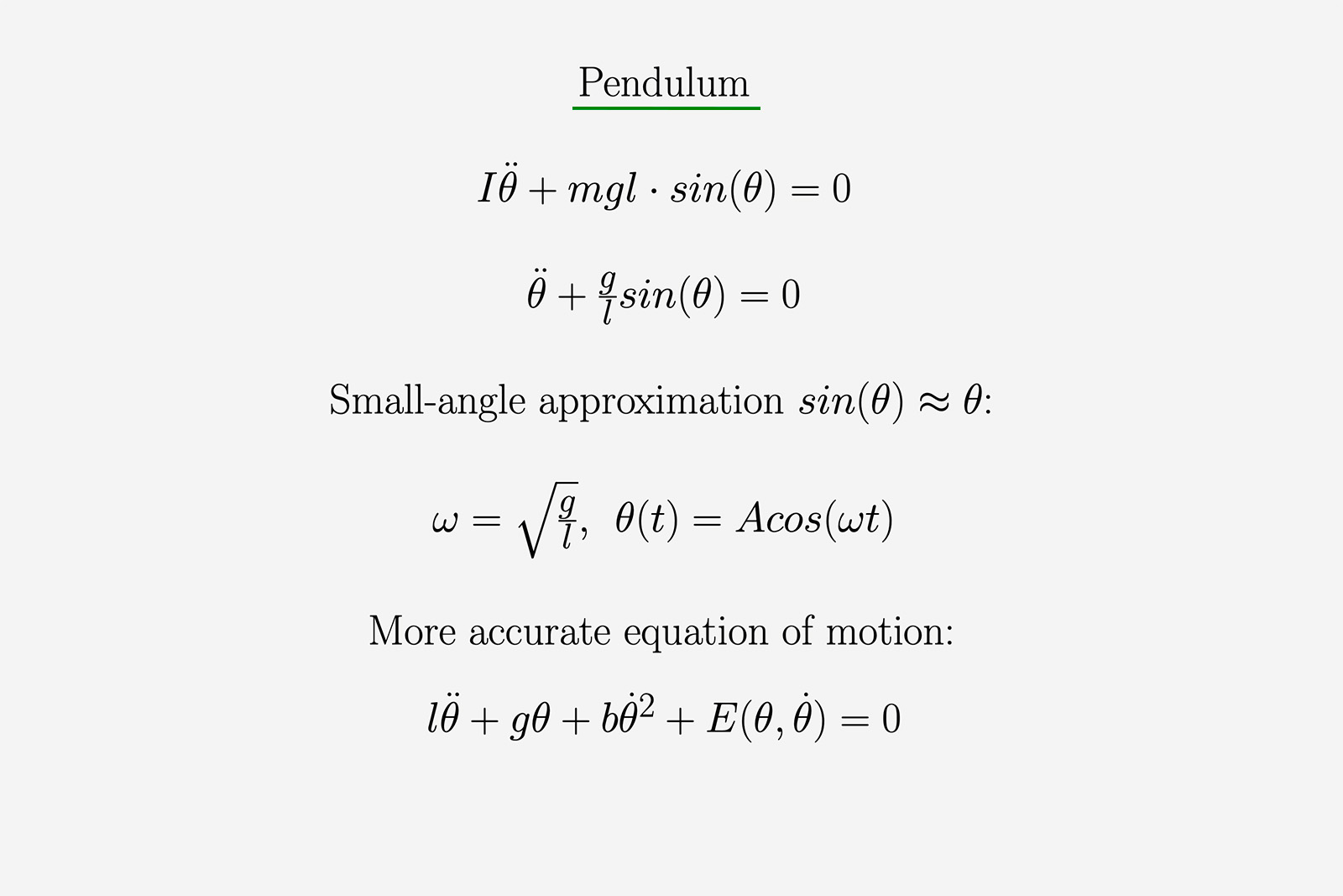
Figure V. Equations governing the free-swinging pendulum.

In order to tackle this issue, we’ll need to make a concession. Well known to engineers is the “small angle approximation” — the mathematically-supported fact that for sufficiently small angles, the sine of the angle is considered equal to the angle value itself. This can be checked by considering the Taylor expansion of the sine function. 

So if we just replace the trigonometrical culprit with the angle, we get a proper equation for an isochronous harmonic oscillator. But herein lies the caveat which ties the idealised model with real-world mechanics: how small is sufficiently small for the approximation to work?

Mathematically, very small means approaching zero. Since we can’t have an almost-zero pendulum amplitude, we could assume anything under 1° should be fine. 

But that is mechanically impossible, since the pivot and air friction dampen the real pendulum, which requires an escapement to add back lost energy and set the going train discharge speed. The escapement needs to have some geometric liberty for its work sequence — unlock, impulse, lock. Working between -1° and +1° is practically impossible. 

This is why in real world an angle of 5° is considered a sufficiently small yet practical amplitude. For this small of an oscillating amplitude, the inherent isochronal defect is insignificant. 

If we accept the small-angle approximation, the natural frequency becomes dependent only on the gravitational acceleration and the pivot length of the pendulum. This comes with its own unexpected caveats: the gravitational “constant” g is in fact not constant everywhere and the pendulum length is susceptible to slight changes depending on the temperature modifications. 

While usually taken to be 9.81 m/s², g has slightly different values across the globe, influenced by the planet’s shape and even by Earth’s density at a given spot. The constant modifies mostly in relation to the distance from Earth’s center, so should a clock that keeps perfect time around the Equator bulge be moved closer to the North Pole, it would automatically speed up. 

There could be some polynomial function encompassing both the air drag and pivot viscous friction involved with the real functioning of the pendulum. Practical experience and experimental studies shown that about 80% of the energy lost by a swinging pendulum is due to air drag, which dominates over viscous friction. The pivot friction can be further reduced by using alternative fixtures, like knife-edge pivots or blade spring suspensions. A general form of drag here is the third term in the last equation, where b is the air drag coefficient and the angular velocity is squared.

Add to that the recharging function of the escapement, dependent on the angular displacement and velocity and we have a more accurate, but infinitely harder to solve equation of the real pendulum. This additional escapement function is not related to the sinusoidal function for the forced harmonic oscillator model and the resonance phenomenon, which is an important distinction to make.

While the pendulum seems inherently doomed to not be a good timekeeper, large standing clocks can be refined to such degree that a regulator can keep time to about one to two seconds deviation per month. Some historic pieces from Riefler or Strasser & Rhode are known to perform even better. 

The trick is building large and heavy pendulums, which can be equipped with temperature compensation gridirons. Although mass plays no part in the pendulum equation of motion, the added inertia helps it store more kinetic energy, thus becoming less susceptible to outside disturbances. The early mercury and later Invar temperature compensation devices made sure that the pendulum length remained sensibly the same over a wider range of temperatures. 

More extreme implements include sealing the pendulum in a vacuum or reduced-pressure chamber, as to eliminate any barometric influences and the air drag.

Very precise escapements (like the Riefler, Strasser or various gravity escapements) are used, which provide consistent recharging power close to the equilibrium point. Crafting such precision regulator clocks was and remains a daunting task.

The sprung balance

We just saw that regular pendulums are not really inherently fit for being good timekeepers. Moreover they are completely dependent on gravity to always point in the negative vertical direction, meaning they’re dependent on orientation. Pseudo-isochronous precision clocks only work well if completely stationary relative to the ground. 

When Huygens invented the spiral hairspring and paired it to an inertial body, the scientist managed to translate the linear harmonic oscillator model into an exact rotational system analogue. This is why his version of the sprung oscillator is the only one which actually worked, compared to other failed attempts of his contemporaries. 

How Huygens realised that this particular setup would work this well is unclear. Today we can easily check the system’s validity using calculus, but the method was introduced by Newton only much later, along with his laws of mechanics.

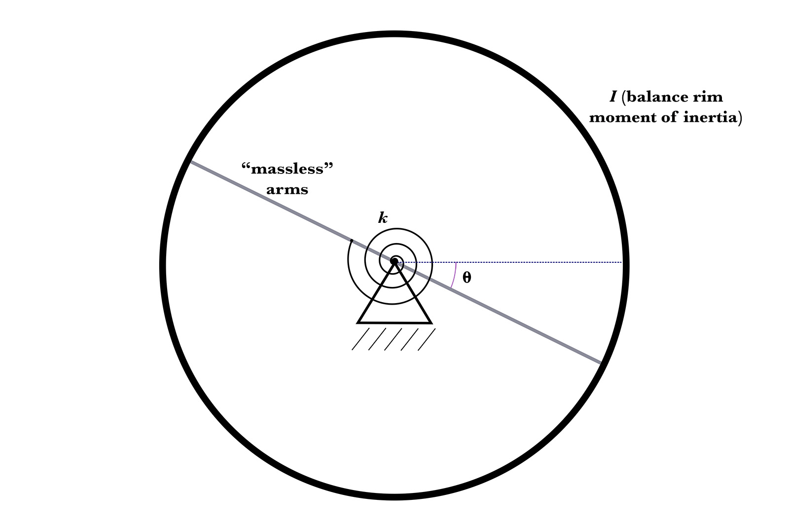
Figure VI. Free-body model of a sprung balance.

Let’s now look at a simplified model of an ideal sprung balance oscillator. Figure VI shows the balance wheel modelled as a circular rim with massless arms (for any real balance can be found such an analogue retaining the same total inertia I) paired to a spiral spring of angular stiffness k. Using the same Lagrangian/Newtonian method as before, we retrieve the following equation of motion on the first row of Figure VII a.

The simplified expression on the second row has the same form as the very first equation of motion for a harmonic oscillator from back in Figure III. We can see the pulsation ω is just a function of the spring’s angular stiffness k and the balance’s inertia I, and the harmonic oscillator solution of angular displacement holds. 

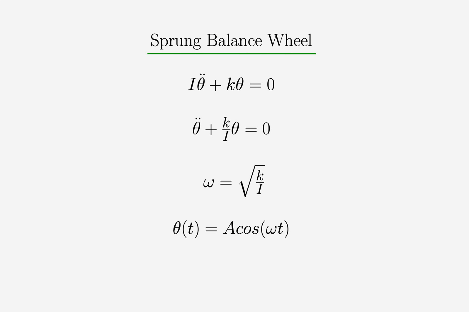
Figure VII a. Equations governing the sprung balance.

This means that the ideal sprung balance is inherently isochronous, compared to the pendulum. Then why does the term isochronism defect come up so often when speaking about balances?

Simply because there are many environmental factors that make real balances stray from the ideal model. Much like with the pendulum, a more faithful equation of motion (Figure VII b, first row) would include a function of the viscous friction and an escapement function, defined again in terms of angular displacement and velocity. Although the system is affected both by the spring’s constant intermolecular friction and air drag, Thierry Conus concluded in his doctorate thesis on escapement design that viscous friction dominates over the other two in terms of dampening a sprung oscillator lubricated at the pivot ends. 

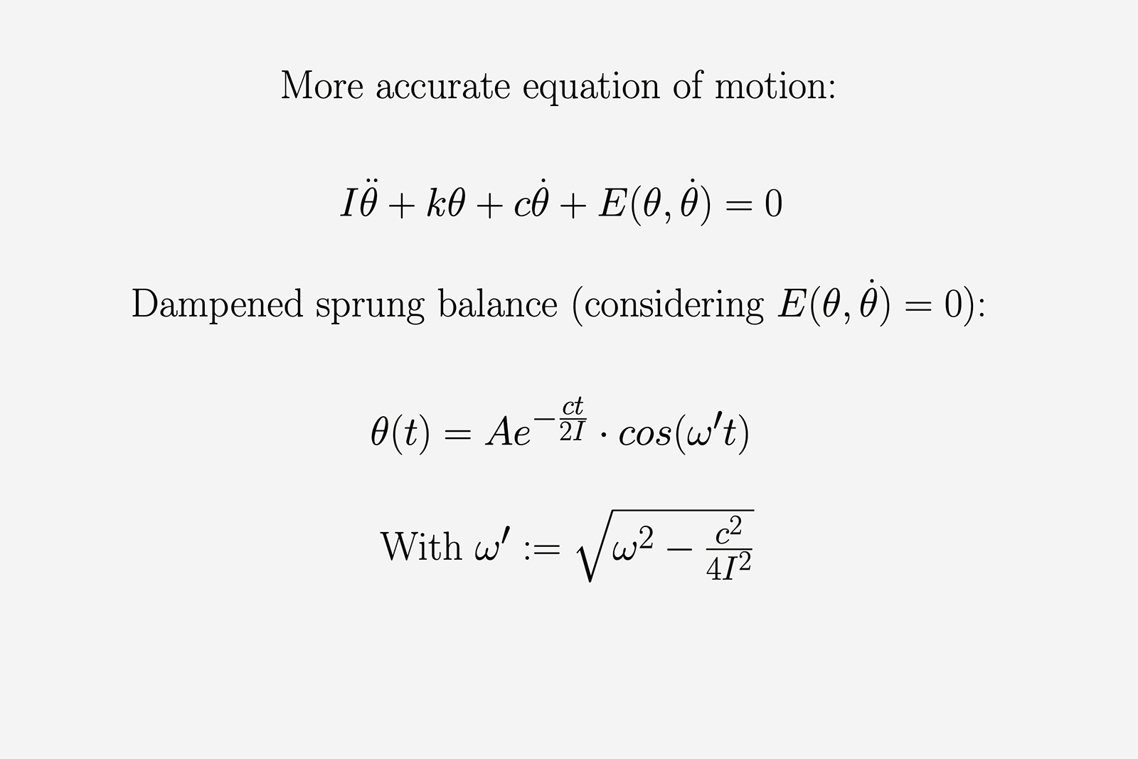
Figure VII b. Some more accurate equations.

If we’d just remove the abstract escapement function, we are left with a textbook dampened harmonic oscillator (Figure VII b, last two rows), which once started will go through progressively weaker amplitudes, eventually stopping. The equation can be solved, with the solution shown in the penultimate row. Compared to the harmonic oscillator, there is an additional exponential decay factor. 

The dampened oscillator is no longer truly isochronous — its pulsation ω’ is smaller and dependent on the viscous friction coefficient. Yet, its expression remains objectively independent of amplitude, so from a watchmaker’s point of view a dampened sprung balance is still isochronous. 

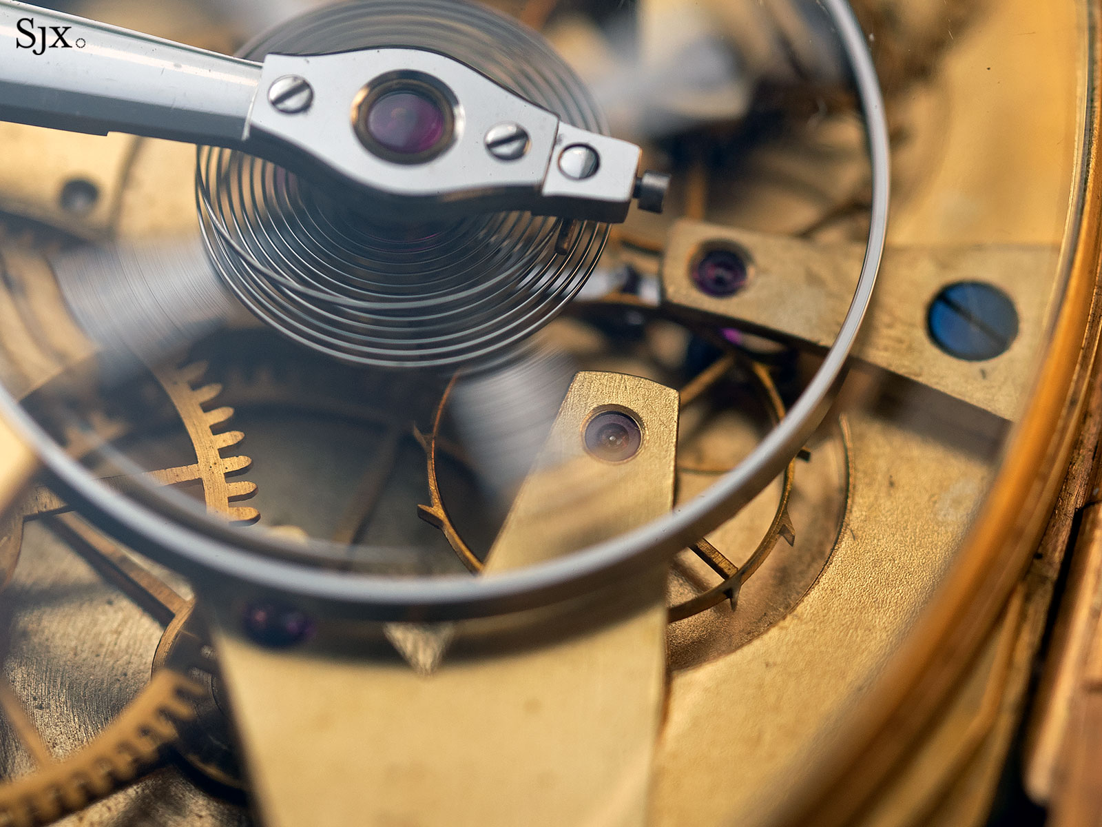
There is also the issue of uneven breathing of the hairspring coils, which adds some residual torque to the balance pivot, pushing its ends harder against the jewels in specific patterns — which generates additional wear and friction. We covered the subject of overcoils and their effect on improving isochronism more broadly in a previous story. 

The impractical influence of the escapement

It appears that the greatest disruptor of the sprung balance is what keeps it beating: the escapement. Artisanal watchmakers and theoreticians alike are familiar with the term “escapement defect”. This refers to the way the swift interaction between the swinging balance wheel and the escapement affects the harmonic motion of the former.

Although the engagement in a Swiss lever escapement takes no more than a few milliseconds, its phases have different influences on the oscillator. First there is the unlocking phase, where the escapement poses some resistance to the balance. The impulse starts being impelled before the equilibrium point of the hairspring and keeps being impelled after the quiescent point. Lastly there is a short interval when the balance impulse roller is still in contact with the anchor, guiding it to the banking, although the escape wheel is going through the drop phase and loses contact with the impulse pallets. 

The unlocking robs the balance of some of its energy, increasing momentarily its natural period T thus causing a loss in rate. The impulse impelled before the equilibrium point shortens the period and causes a gain, while the impulse given after the equilibrium point along with the final part of anchor engagement both cause a loss. 

Summing everything up gives us a global loss of rate, or an increase in the swing period T. Taking into consideration that this disrupting action takes place each alternation, its effects are doubled over one full oscillation (two vibrations). 

Looking at the detent escapement, its unlocking action is softer compared to the Swiss lever, thus causing less of a loss. The detent’s radial impulse is given after the equilibrium point, leading to another loss. Overall the detent escapement causes an increase in the swing period T, thus a loss in running rate — but less so compared to Swiss lever, since this action happens only once every full oscillation and has a lighter influence.

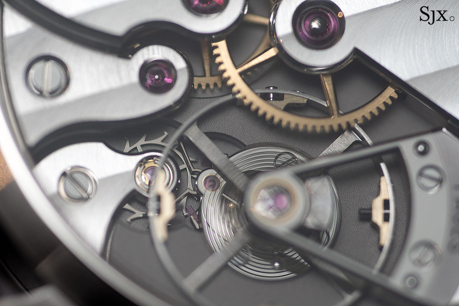
One escape wheel inside the Daniels’ Double independent escapement, which can be seen as a mirrored detent escapement.

This brief escapement analysis also hints at why the real sprung balance is not a traditional forced oscillator model, since the escapement action (or function as we’ve called it before) is not sinusoidal and there can be no question about resonance between two vibrational systems. 

In knowing that an escapement generally causes a loss, the watchmakers can in fact adjust the sprung balance, so that its natural period is slightly decreased. So even though a movement nominally beats at 4 Hz with a stated period of 0.25 seconds, the oscillator’s swing might be shortened to a 0.249-something period (equivalent to 4.01-something Hz). This countering of the escapement-induced loss is a component of the “adjusted for isochronism” designation on high quality movements. 

The issue with this adjustment is related to the decreasing barrel power, which delivers less and less torque to the escapement as it unwinds. As such, the particular effect of the escapement phases on the balance is disturbed, so the isochronal correction is insufficient. With the isochronism defect still present (although to a lesser extent with the initial adjustment), the variance in balance amplitude hinders the accuracy. 

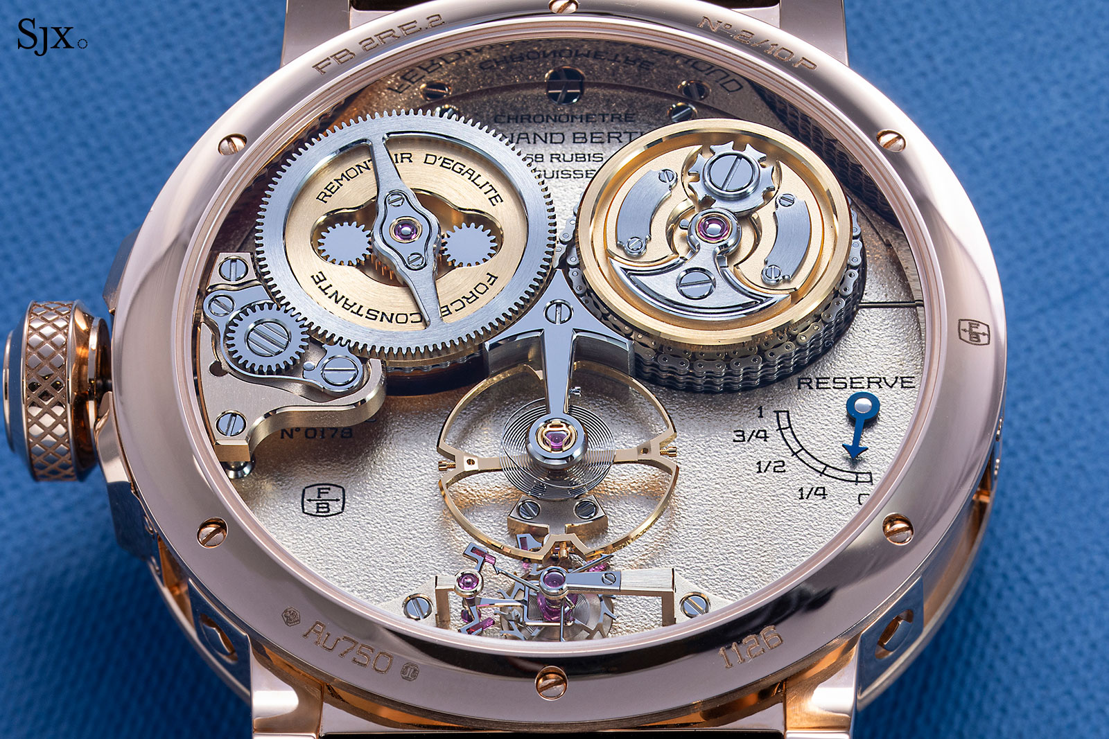
Watchmakers have long attempted to counter this problem by modulating the torque delivered to the escapement. Historic solutions include the fusee and chain, the remontoire, and the simple stopwork. Conveniently, all three of these systems can be observed at work in the Ferdinand Berthoud FB2.

In a perfectly isochronous sprung balance, a drop in amplitude would be offset by a corresponding reduction in speed, allowing the oscillator to sweep a smaller arc in the same time as a larger one. But because the escapement disrupts true isochronism, the balance does not fully compensate for reduced amplitudes.

Small defects such as slight poise errors or degraded lubrication, which may be invisible at higher amplitudes, become more pronounced as the amplitude falls. This is why dynamic poising is performed at low amplitudes: uneven hairspring mass, eccentric breathing, or heavy spots on the balance are easier to detect under these conditions.

Some loss of accuracy near the end of the power reserve is unavoidable, even in the best-made timepieces, because isochronism defects are inherent to the traditional construction. A more subtle, wristwatch-specific disturbance arises from the oscillator’s vulnerability to certain angular accelerations.

For example, if the watch experiences a precisely timed acceleration around its axis, the balance may momentarily gain or lose amplitude. This is rare, but the weakness exists and can account for occasional unexplained rate deviations. Higher frequencies help mitigate this by reducing the sensitivity to such accelerations.

Conclusions and future perspectives on oscillators

While the hairspring–balance oscillator remains the most suitable portable timebase for mechanical watches, it still has limitations. And although the traditional sprung balance is unlikely to disappear anytime soon, major brands and academic researchers have been exploring alternatives for many years.

Horology enthusiasts might already be familiar with the so-called “monoblock” oscillators crafted from silicon. Mainstream brands like Ulysse Nardin, Zenith and Frederique Constant have already commercialised escapements with flexural pivot oscillators, which integrate elasticity, mass and virtual pivots inside one MEMS device. The “monoblock” oscillators work by exploiting flexible guides (also known as “compliant mechanisms”) and their virtual elastic pivot points created by intersecting slim spring blades.

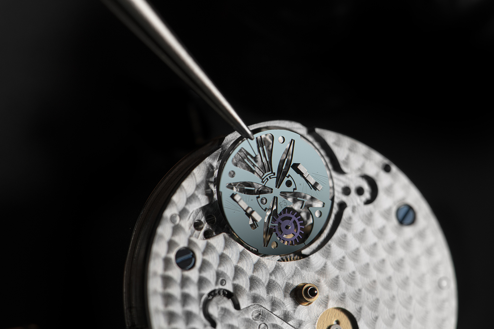
Frederique Constant monoblock oscillator. Image – Frederique Constant

While the theory on flexural pivots is still advancing, the already available models seem promising enough, although this breed of oscillators is still far from perfect. Their “stroke” (amplitude of motion) is limited and they usually generate a parasitic shift of the virtual center of oscillation. They require their own special isochronism tuning devices and the most conceptually advanced systems are still in the research phase.

Another promising oscillating mechanical timebase was presented by the EPFL Instant-Lab horological research laboratory in Neuchâtel: the Iso-Spring. The system doesn’t need an escapement and relies on the intrinsic isochronism of elliptic trajectories. A working clock has been running in the Neuchâtel town hall for a number of years now, but that iteration is still affected by gravity, much like a pendulum.

Earlier this year a PhD degree was awarded by the university to a researcher who created a wristwatch-compatible Iso-Spring oscillator. A working prototype adapted for a generic ETA powertrain was built and showed promising results; future developments of this system could be intriguing.

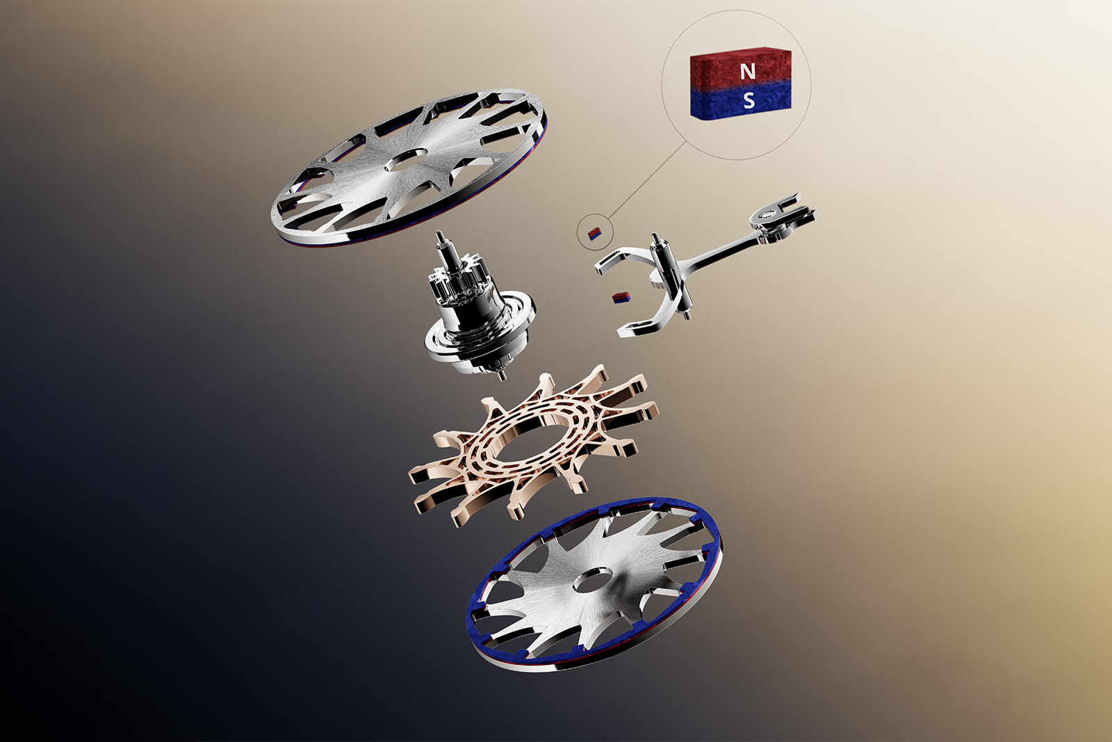
The Breguet magnetic constant-force escapement. Image – Breguet

Interestingly, even in the age of A.I., the search for improved mechanical oscillators remains active. Breguet recently unveiled the Expérimentale 1, a 10 Hz tourbillon driven by a magnetic constant force escapement. Omega introduced the Spirate fine-regulating system a few years ago, and Rolex presented its Dynapulse escapement earlier this year. That major brands continue to refine mechanical timekeeping — alongside specialised research in academic institutions — suggests an encouraging future for the machine with a ticking heart.