In a past story, we explained how multiple mainspring barrels can be paired in parallel or in series, for either lengthening a movement’s power reserve or increasing the torque discharged into the going train. In this article we expand on this topic to analyse the inside of the barrel by exploring how mainspring size balancing influences the torque output and power reserve.  

Enthusiasts tend to throw around the loosely-defined term “mainspring packing” — especially when criticising a movement’s unsatisfying power reserve. This term refers to how a watchmaker can get a higher power reserve by balancing a spring’s dimensions and the space it occupies inside a barrel. While this sounds simple, the reality is more complicated. 

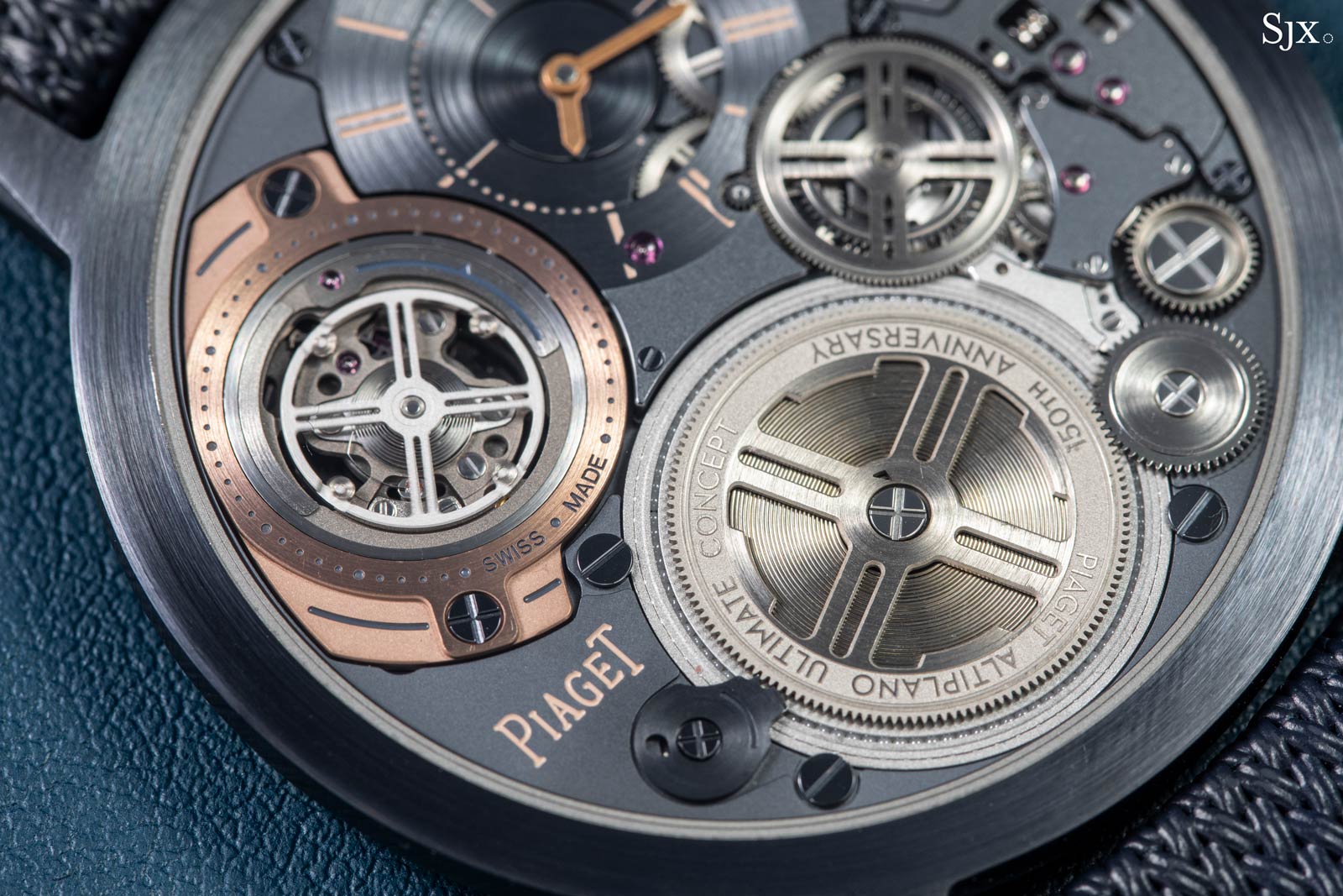
Skeletonised barrel showing the tight coiled mainspring inside the Piaget Altiplano Tourbillon Concept.

In order to set the record straight, it’s necessary to analyse the topic thoroughly. This requires getting a bit technical, but an interpretation is included for those less interested in the underlying maths. This theory-heavy deep-dive tries to unravel the concept of mainspring packing and explores why optimisation is not a very straightforward business.

The core elements

This section covers the basics of mainspring and barrel geometry and establishes their relation with power reserve and torque. In order to see how specific dimensions affect both torque and power reserve, we will resort to some known functions and a little geometrical reasoning. Equally, we need to take into consideration that the available space inside a barrel is finite. Since it is spanned by the coiled strip, sizing the mainspring implies some trade-offs. In short, one can either have a thick mainspring with few coils, or a long spring but with thinner coils.

The analysis will mainly revolve around these four notations: L – the total length of the coiled spring; e – the thickness of the spring, N – the number of developing turns of a mainspring, from fully wound to fully depleted; K – the stiffness of the coiled spring of rectangular section.

The running power reserve is in fact analogous to the number of developing turns N. A large N value is synonymous with a long power reserve. In order to see how N really scales with the two variables e (spring thickness) and L (spring length), we start off with some geometric considerations.

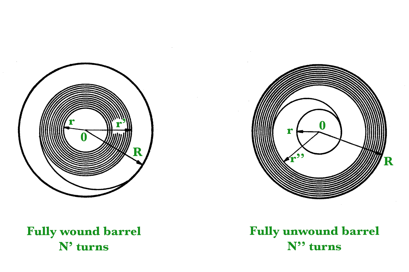
Figure I. The mainspring in fully wound and unwound states.

Figure I shows the two extreme states (wound and unwound) of a mainspring barrel. Since the coils physically span the barrel space, we can find by geometric reasoning both the number of turns of full charge N’ and the number of turns of a depleted charge N”. R is the interior barrel radius, measured from center to wall.

The other radius r is not the arbour radius, but rather the realistic radius of the innermost mainspring coil. A spiral spring would fracture or permanently bend, should it be coiled fully around the barrel arbour. As such there is an interior limiting factor here, a circular area of radius r that will never be occupied by the spring. 

The complete mathematical reasoning is shown bellow in Figure II, where we link set radiuses R and r to the number of turns N — which then gives us the final expression of available turns function N in terms of just e, L, R and r. 

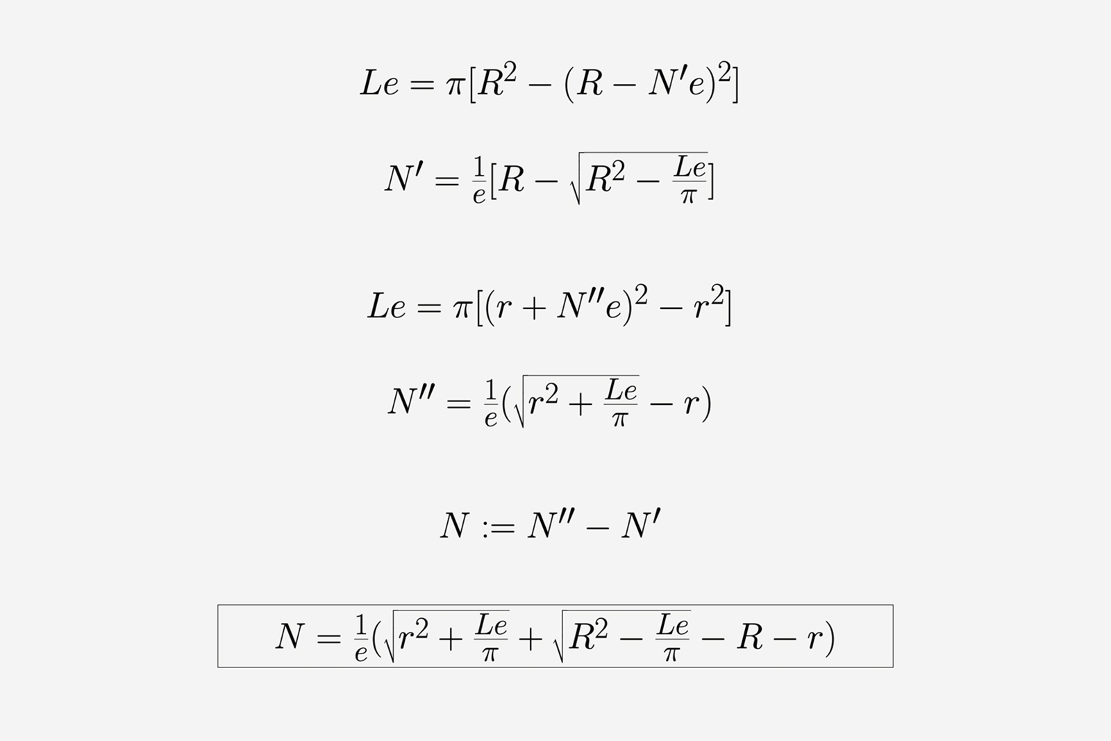
Figure II. Deducing the total number of developing turns.

For the barrel torque, we will refer to the known formula of elastic moment for a coiled spring of rectangular section, shown in Figure III. The formula K shows the stiffness of the system. This value multiplied by an arming angle gives the torque discharged into the going train. Young’s modulus E and the height of the spring h are treated as given constants in this analysis. We will refer to K as the stiffness function while conspicuously doing away with the complete torque expression involving the arming angle, since that is irrelevant to the spring geometry we’re considering.

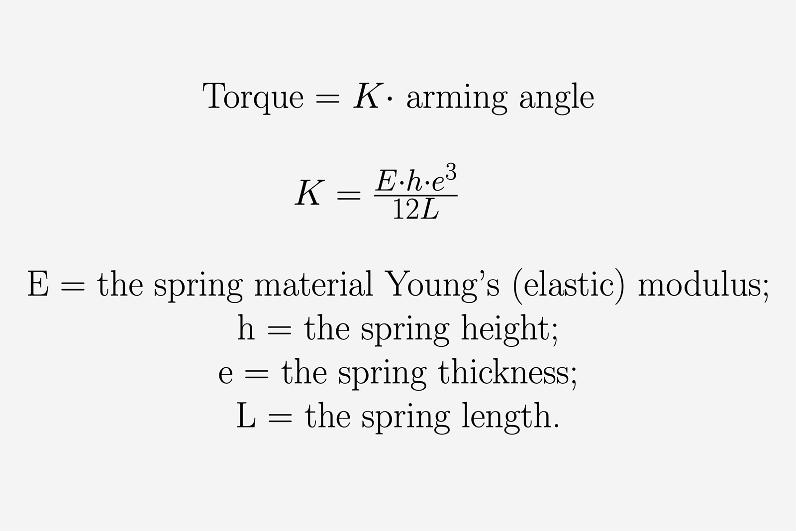
Figure III.

Thus we have established two functions, each dependent on pairs of (L, e) and related to either the torque of the mainspring or its running time. Our goal here is to find some expressions for (L, e) which give us (separately) the largest stiffness K and the longest running time N and see if and how those values relate to each other. And there is no better tool for it than calculus. 

A failed initial method of approach

This section describes my first method of approaching mainspring size optimisation, which ultimately failed. When thinking of getting the best results for L and e pairs, I resorted to a straightforward method, making use of the equations established earlier. Later I realised the approach was flawed, but the fact that it failed is significant; it tells us that balancing mainspring sizes is a more layered matter that it initially appears. The failed experiment is covered in the following.

In multivariable calculus (where two independent variables influence the same equation) there exist constrained optimisation problems which are most easily solved using the method of Lagrange multipliers. 

An example of such an optimisation problem is the following: what is the maximum possible area of a rectangle of unknown side lengths, knowing that it has a set perimeter. This means that the sum of its sides is some fixed constant (the constraining function) and we need to find the optimal values so that our rectangle’s area reaches a maximal value. 

This sort of problem is usually solved by using Lagrange multipliers, as we try to find some linear dependence between the gradient vectors of the given and constraint functions. Leaving the mathematical jargon aside, this is usually a very useful way of finding maximal (or minimal) solutions to a multivariate expression. 

This method initially appeared to cater well to the mainspring problem. We look  to find both the optimal L and e for either a long power reserve N or a stiff K— all while under the mutual geometrical constraint of the finite barrel space. In other words, we want to find optimal pairs of mainspring width e and length L by separately maximising the N and K functions with regard to the finite available barrel space. 

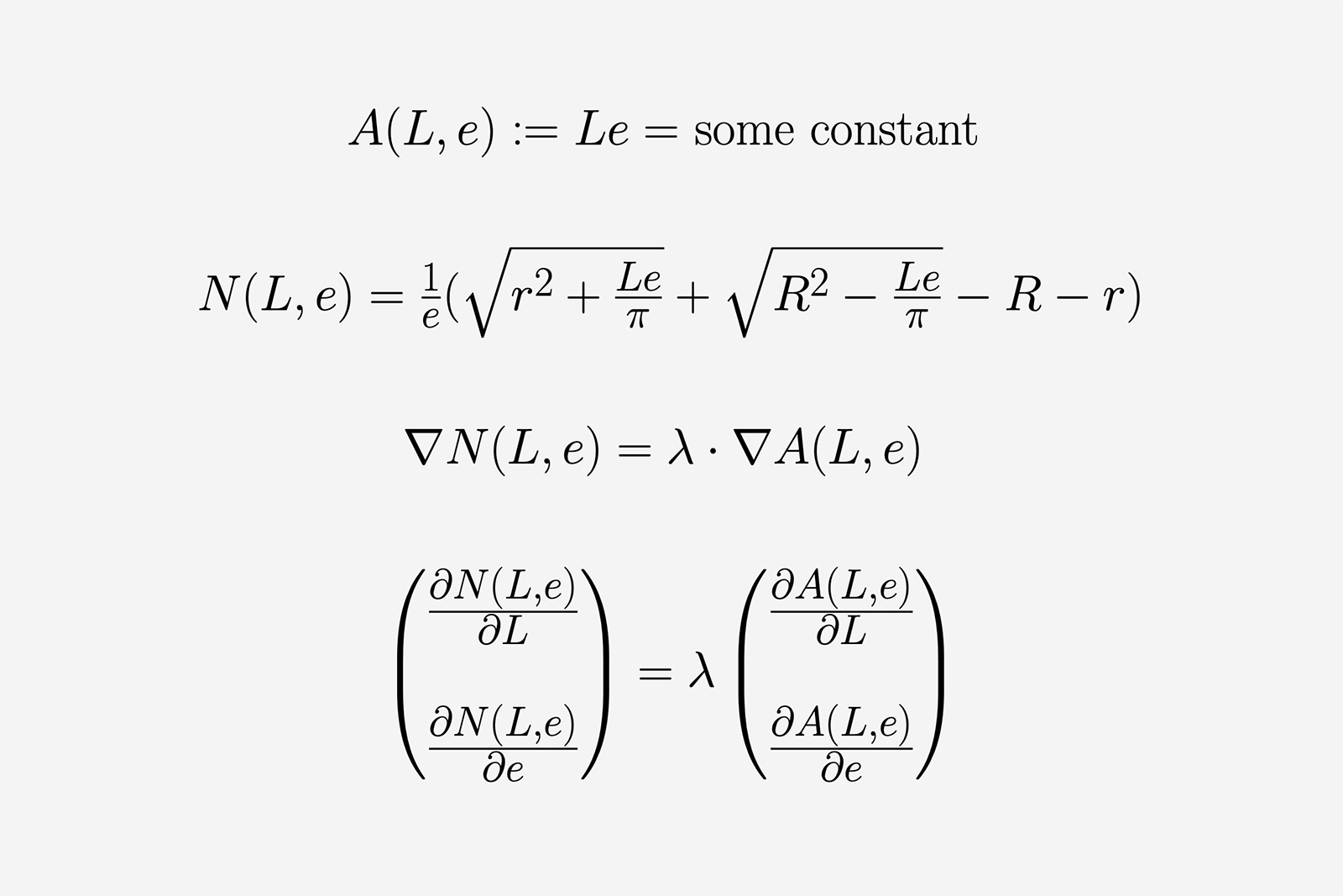
Figure IV. The multiplier method setup.

For those interested, the equations above in Figure IV show how the system was initially set up. First we have the two gradient vectors, with the partial derivatives of N and area function, the product of e and L. Then a suitable scaling parameter λ is found — provided that the two vectors are indeed linearly dependent. The equations are then solved, hopefully yielding the pair (L, e) which serves as an extremum point for our N function. The process is a little abstract and unrelated to horology, but useful nonetheless.

The Lagrange multipliers method yielded plainly unusable results. The constraining function relies on a simple geometrical fact: the area spanned by a coiled mainspring of rectangular section is Le (length times thickness), which remains constant. But what is, in fact, that constant?

Looking back to Figure I, it looks like it might just be the difference between the area defined by R and the small circle area defined by r. This couldn’t be more incorrect, since there needs to be some space left for the spring to move around, from wound-to-unwound and vice versa. This free space being an unknown value in itself is one of the reasons the Lagrange multipliers reasoning fails. 

Applying the method only yielded the degenerate result of N=0 (or e going to infinity). This was traced back to an engineer’s worst nightmare — mathematical rigour. After a more thorough analysis of N as a function, it appears that it is inherently unfit for the Lagrange method, due to issues having to do with bounds and regularity. 

The nightmare worsened when I noticed the same fault with the K function as well. In other words, there is no way to get optimal pairs of both L and e for either function. 

This approach’s failure does tell us something though: the relation between L, e, K and especially N is not a straightforward one, and there is no instant wonder result for building a theoretically optimal mainspring. Thus we proceed to investigate each function, piece by piece. 

Back to more classical approaches

This section takes a different approach at studying how mainspring length and thickness influence both the stiffness and power reserve, by reviewing some of the initial assumptions. Looking back, there was one other error which plagued the reasoning: I initially considered the spring width e a true variable, to be found in the same manner as L. In doing that I overlooked the fact that e is realistically constrained by stress/strain relations. 

A thick beam can’t bend very much without permanent plastic deformation and even fracture, and we need many circular coils for a spring. Surely there must be some hard constraint on the strip thickness, hopefully also related to the barrel system geometry. There is one parameter, r, which is a strong contender, since r is practically linked to the elastic limit of the innermost coils. 

Leopold Defossez suggests that a ratio r/e of 16 works very well as a constraint, since the spring deformation during coiling-uncoiling around the arbour remains elastic. A ratio of 16 just means that the interior radius is sixteen times larger than the spring thickness. The ratio implies a direct relation between e and the inner barrel arbour radius r — meaning e is no longer a variable, but linked to parameter r.

In seeing that e is no longer a random variable, I resorted to just deriving N in terms of L (which here is possible, all rigour considered). Setting the derivative of any function to zero gives an extreme point of the function, which can be either its minimum (for convex functions) or maximum (for concave functions). Checking that N is indeed concave, when setting its derivative to zero (first row) we should find both the peak of N and its root L. This actually yielded a good result — the expression of L in terms of R, r and e (second row) which gives a maximum value N (fourth row). The computations are shown below, in Figure V.

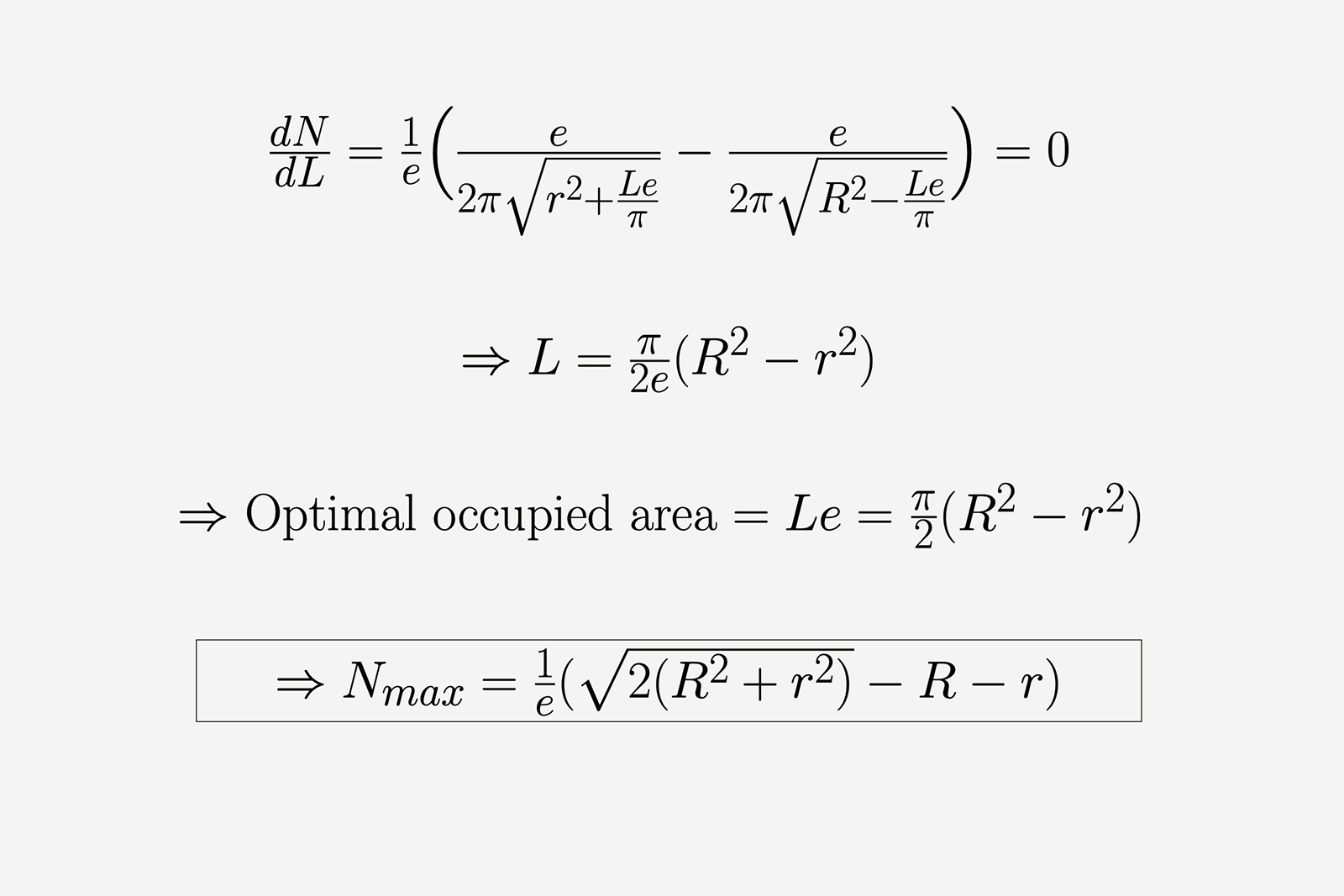
Figure V.

Also, when multiplying this newly-found L by e (third row) we get the barrel area the spring occupies — which is exactly half of the total area available. Plugging this back into N gives us the maximum power reserve given by a mainspring of thickness e, lodged inside a barrel of R and r. The expression is consistent with that found in textbooks, although newer ones don’t go to the length of explaining its provenance. 

And now let’s consider the r/e ratio more thoroughly. We’ll call it α and rewrite all our important expressions in terms of it. We write N, L (specifically the expressions we just derived) and K in terms of α and immediately see some interesting things. 

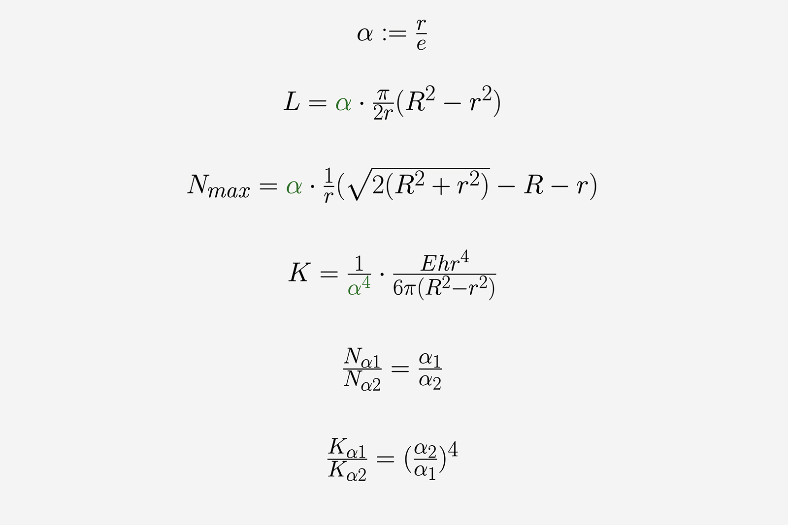
Figure VI. Introducing α and ratios.

As α goes up, so does N in a linear fashion (third row). At the same time, K goes down very fast, since the expression includes the fourth power of the inverse of α (fourth row). It seems, pleasingly, that some relation between N and K is only dependent on this value α, all other factors being kept constant. 

The beauty of this is how all our relations remain valid, regardless of α’s value. The area spanned by the mainspring remains the same, and N and K only change with regard to α. By plugging in different numbers, we get the the maximum power reserve and the associated stiffness for the same set of constant construction parameters — R and r. In other words, we are now really talking about “mainspring packing”.  

The last two rows of the  equations above show the ratios between two Ns of different α and two Ks of different α. When keeping the R and r constant, both equations reduce to ratios in terms of just α. This gives us an interesting system to play with. 

While in the past the lowest admissible value of α was 14, due to advancements in material science and manufacturing, the lower limit today is more in the vicinity of 10. By title of example we can consider α to be 12, 14 and 16 — and observe the variance in the running time and stiffness of differently sized mainsprings spanning the same barrel.

Discussion of results

This section concerns the final results of our analytical endeavour. We see how by incrementally varying the thickness of the mainspring, both the power reserve and stiffness are affected (but very differently). The reduced ratios below should help in explaining the interesting relationships between different “mainspring packings”.

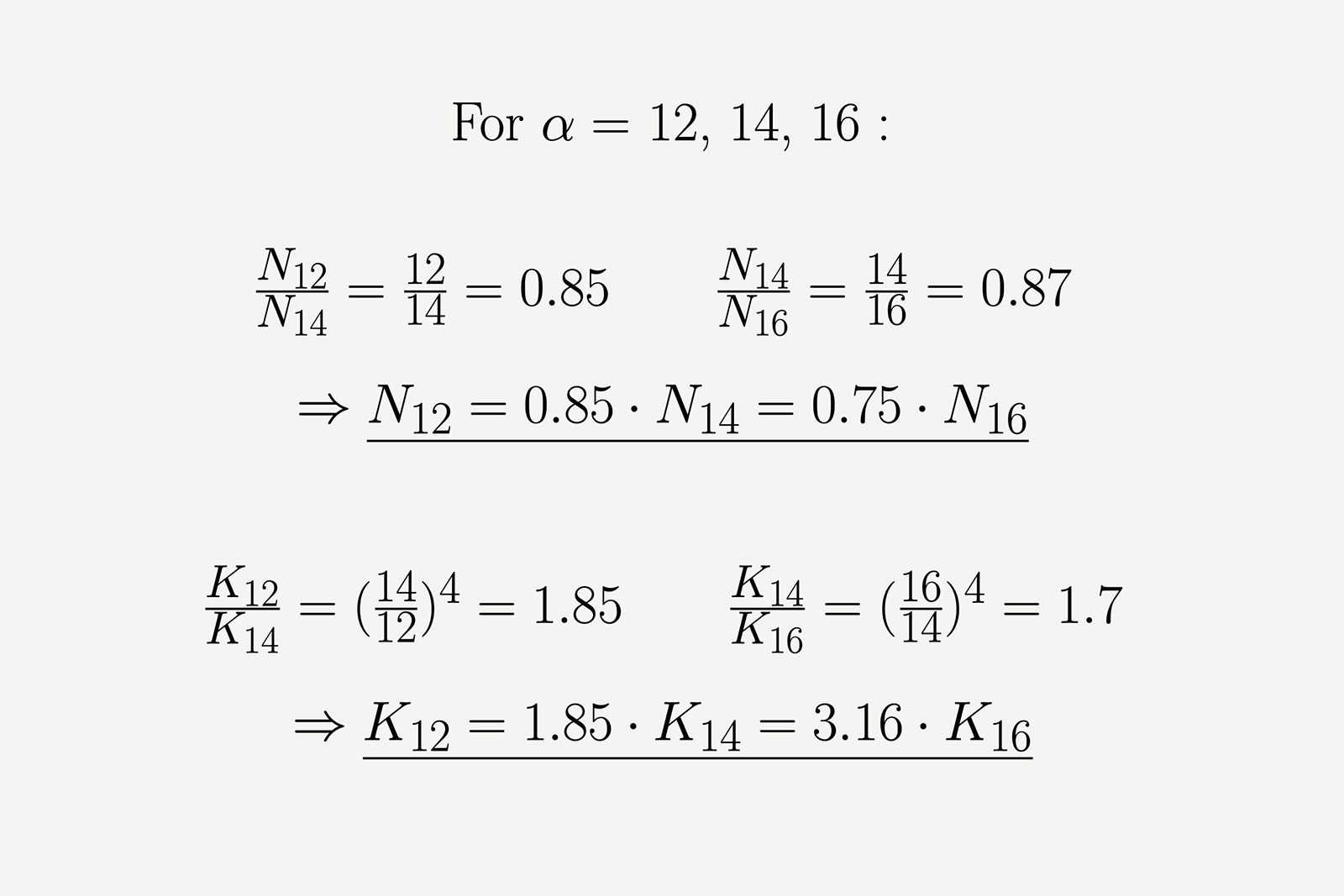
Figure VII. Balancing power reserve and torque.

Figure VII shows K12 is 85% stiffer than K14, and a staggering 216% stiffer than K16. This means that a mainspring of thickness r/12 is more than three times stiffer than another of thickness r/16. Now let’s look at the different ratios of N. Here the ratios are not as sharp; N12 is 85% of N14 and only 75% of N16.

The ratios are indeed telling. Varying α from 12 to 14, decreases the power reserve by 15%, but increases the potential torque output by 85%. It looks like a fair trade, since subtracting 15% from a standard power reserve of say 72 hours leaves us with around 61 hours. This still is a comfortable running time and the barrel torque is almost doubled. 

Considering an even sharper variation, from 12 to 16 makes for a 25% reduction in power reserve, but offers over three times the torque. So if the slim mainspring would run for 72 hours, the thicker one would only run for about 54 hours, while exerting thee times the torque. In this case, the stiffer mainspring would be just one third thicker than the slim one — not a huge variance, but with great effect. 

In real life, when going about building a mainspring barrel, watchmakers and engineers probably start by fixing R, since it is constrained by other movement and gear train dimensions. Then the desired N number of developing turns is set. The inner radius r can be then found early on as well and usually is one fourth to one third of R. Based on that, α is then determined and some e is found to satisfy it. This makes sure N is indeed maximal for the imposed barrel radius R. The spring however doesn’t have the highest torque output possible.  

This initial result can be tweaked for movements which prioritise a higher torque output: chronographs, perpetual calendars, tourbillons etc. In that case α can be slightly decreased by raising e, leading to a healthy gain in mainspring stiffness, while sacrificing just some of the power reserve. 

As the ratios show, any increase in thickness can go a long way in increasing the spring stiffness, while the power reserve is not decreased too much. The relation between r and e gives quite a large degree of freedom (α is not set to natural numbers only), so there is a wide theoretical range of torques and power reserves that can be obtained from one barrel size. In the real world, watchmakers are only limited by the choices offered by spring manufacturers, who produce springs in normalised sizes.

Another important takeaway is that there is a maximum number of developing turns associated with any given barrel size. So for any barrel to have the longest possible power reserve there can be found some exact values. This is not the case with stiffness. Function K has no maximum in terms of neither L nor e. So trying to get a stiffer spring for stronger torque always means straying away from the “perfect” power reserve for the given barrel size.

Limitations of the analytical method

As is often the case with purely theoretical reasoning, the results and conclusions drawn may not line up exactly with empirical evidence. For example, due to experience, watchmakers tend to fill as much as 55% of the interior barrel space with the coiled mainspring, while theory suggests that 50% is optimal. The difference is minimal, but deviates from the theoretical result due to practical experience. Watchmakers usually chose a length that is 1.2 times larger than the analytically determined optimal L, which conceivably leads to the increase in occupied barrel space. 

There is also the issue of uneven development of the coils inside the barrel. Much like with hairsprings, the mainspring doesn’t uncoil truly concentrically, leading to a real-life number of developing turns that is smaller than the intended N. To account for this behaviour, a small corrective factor (about 0.002 to 0.004) is added to e during the computations.  

To end this lengthy analysis, I must say this only scratches the surface of the quest for mainspring barrel optimisation. Engineers and watchmakers have to take note and study many other aspects of the motor organ, from spring material fatigue and magnetism resistance to lubrication, along with barrel wall thickness and side pressures on the wall and inner arbour. An often overlooked component of the mechanical watch, the mainspring barrel is quite a fascinating system which is still being actively improved by movement constructors.